Two new Excel functions replaced every pivot table I used to build

For years, pivot tables have been my go-to for almost every data summary task in Excel. Over time, I got pretty good at them, field lists, value settings, the whole ritual, but they never quite felt like the right way to do things. Then I found a new Excel function and stopped building pivot tables at all.

Microsoft quietly shipped two new functions in Excel called GROUBBY and PIVOTBY. These two functions do everything I was using pivot tables for, and they do it in a single formula that types into a cell like any other.

Pivot tables are powerful—but they're also clunky

The friction of building, refreshing, and maintaining summaries manually

Pivot tables have one fatal flaw that always bothered me: they don't refresh themselves, and it gets worse the more serious your work gets. You can make a beautiful summary, share it with someone, the source data gets updated, and unless someone remembers to manually refresh the table (which someone always does), suddenly your summary is lying to you. In a fast-moving spreadsheet where source data is constantly being updated, that's a major bottleneck that makes pivot tables borderline useless.

The other problem is that pivot tables live outside your formula logic. You can't easily feed one into another function, chain it into a FILTER or SORT, or use it as a dynamic source for a chart that's also pulling from the calculated data. They're powerful, but isolated in a manner that makes them much less useful.

GROUPBY and PIVOTBY fix both of these problems. And now that Excel finally speaks Regex, it can clean up the data you had to previously fix by hand, too.

GROUPBY feels like a pivot table in a formula

Creating dynamic summaries without leaving the worksheet

Think of GROUPBY as a pivot table that lives within a formula. In its most basic form, it requires three things: the column you want to group by, the column you want to aggregate, and the function you want to use. That's it.

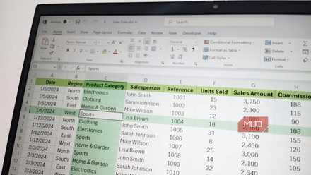
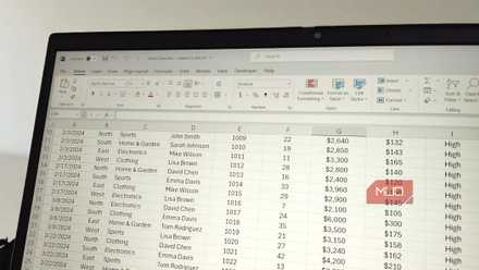
Let's say you have a sales dataset and you want the total revenue by product category, you write something like =GROUPBY(C2:C500, E2:E500, SUM) and hit Enter. Excel will automatically make a complete summary table right into your sheet with category names in one column, totals in the next, and it updates the moment anything in your source data changes. No need to manually refresh every time.

What makes it even more useful is that you're not limited to one formula. You can use AVERAGE, COUNT, MIN, MAX, MEDIAN, or even text aggregation functions to create tables showing all sorts of data. Text aggregation functions allow you to combine text values from multiple rows into a single summarized cell — something that pivot tables can't do at all.

You can also sort the output directly inside the function, filter which rows get included, and control whether totals appear. All of these tasks would require extra steps or helper columns when working with pivot tables, but they're simply arguments you pass inline with GROUPBY.

PIVOTBY takes it one step further

Building cross-tab reports using formulas instead of separate objects

GROUPBY gives you a one-dimensional summary. You get categories down the rows and aggregated values next to them. For two dimensions, such as if you need to see sales by product and by month, you'd need PIVOTBY.

PIVOTBY works exactly like GROUPBY but adds a second grouping axis. You give it a row field, a column field, a values range, and an aggregation function, and it builds the full cross-tabulation. For example, consider this:

=PIVOTBY(C2:C500, A2:A500, E2:E500, SUM)

This formula will produce a matrix with product categories down the left and years (or months, regions, or any other axis) across the top, with totals at the edges.

What really makes it stand out compared to a traditional pivot table is that the result is a live, dynamic array. You can wrap it in other functions, use it as a chart data source, or reference individual cells from it with spill notation. Your chart updates when the data updates. Your downstream formulas update, too, and everything stays in sync automatically.

You're not replacing everything

The features and flexibility traditional pivot tables still do better

As easy as GROUPBY and PIVOTBY are to use, they're not perfect replacements for pivot tables in every situation. If you need slicers, timelines, or the ability to double-click a cell and drill into the underlying rows, you'd still want to use the traditional pivot tables. Pivot tables also handle automatic date grouping — breaking a date into years, quarters, and months with a right-click — which these functions do natively. For that, you'll have to wrap your dates in YEAR() or MONTH() yourself, which adds a little extra setup.

More importantly, they're a Microsoft 365 feature, so if you're sharing files with people on older versions of Excel or use one yourself, the formulas just won't work.

Excel's future is formula-driven

Why these functions changed the way I analyze data

If you're building reports that run on the same dataset week after week, the kind where you refresh the source and expect the summary to just be right, GROUPBY and PIVOTBY are much better tools than the usual pivot table.

They're faster to build, impossible to forget to refresh, and composable with everything else in Excel's formula engine. Once you get comfortable with them, going back to the old way feels like an unnecessary hassle.